

Ensuring stability of coastal structures is a necessary step to design long lasting strategies for restoring and protecting coasts. Structures like groines and breakwaters are often built by assembling armour units that can be made by stone or concrete. They are subjected to the dynamic action of waves which implies a continuous stress. The hydraulic processes affecting the stability of coastal structures were extensively investigated and discussed by several authors. Traditionally the design is carried out by using empirical approaches based on the results of laboratory and field experiments, as well as expert knowledge. Some of the approaches take advantage from our knowledge of the physical basis of the inherent processes. Our understanding of the physical mechanisms which control the response of the near shore region to wind, waves and water level changes is in rapid evolution and so are the design methods.
Stability criteria usually make reference to extreme environmental conditions and therefore are related to episodic events. The design is thus based on a frequency analysis of extreme events to determine a design forcing associated to a given return period. In what follows, we will assume that a design wave forcing is available for checking the stability of rock and concrete armour units that may compose a breakwater, a berm protection, a seawall or a groin. We make reference to van Rijn (2016) which is available here.
The problem of initiation of motion of granular materials invested by a flow of water has been studied with laboratory experiments in flumes by Shields (1936). Figure 1 presents a schematic representation of the forces acting on a single particle that is placed over a sloped and flat surface and is exposed to a flow of fluid.
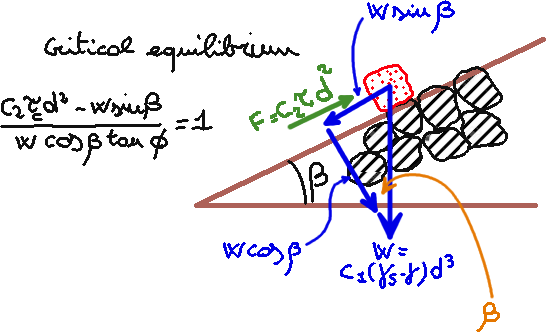
Fìgure 1. Forces acting on a sediment particle exposed to water flow over a sloping surface. τ is friction, which has the dimension of a tension.
The hydrodynamic force tends to move the particle, while its own weight is a stabilizing force. For the case illustrated in Figure 1, the hydrodynamic force is directed upward and therefore the component of the particle weight along the slope is opposing the water flow. Actually, the hydrodynamic force may be directed upward or downward, depending on the direction of the flux. Downward velocity is reduced with respect to upward velocity. More details are provided when discussing empirical formulas for armour units stability here below.
The component of the particle weight perpendicular to the slope, multiplied by tanΦ, where Φ is the friction angle, is also stabilizing the particle. The condition of critical equilibrium is reached when
c2τcd2-w sinβ = w cosβtanΦ
where τc is the shear stress at the critical equilibrium and d is a characteristic size of the particle. Namely,
τc = c1/c2(γs-γ)d cosβ(tanΦ+tanβ)
Here, c1 and c2 are parameters that depend on the shape of the particle. If β=0 and c=c1/c2, one obtains
τc = c tanΦ(γs-γ)d
which can be written as
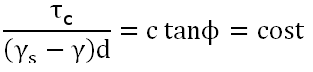
where the left hand side of the above equation is called the Shields parameter and is dimensionless.
Actually, the above analysis is simplified in the computation of the dragging force and in the assumption that the right hand side of the equation is constant and therefore does not depend on flow conditions. A more refined analysis of the process can be carried out through dimensional analysis by means of the Buckingam theorem that states: "if there is a physically meaningful equation involving a number n of physical variables represented by k physical dimensions, then the original equation can be rewritten in terms of a set of p = n - k dimensionless numbers constructed from the original variables". In our case, the physical variables are τc, (γs-γ), ρ (mass density of sea water), d, v (velocity of fluid particle). Since the above variables can be expressed in terms of 3 dimensions, namely, length, mass and time, one obtains p = 5 - 3, namely, the process can be expressed in terms of two dimensionless numbers. It can be proved that the first one is the Shields parameter τc/((γs-γ)d) while the second one is the particle Reynolds number Re* = (u* d)/ν, where ν is the kinematic viscosity of water and u* is the shear velocity which can be expressed as
u* = (τ/ρ)0.5
where τ is friction. Therefore one obtains that τc/((γs-γ)d) = f(Re*)
which means that the Shields parameter is actually not constant but varying with the particle Reynolds number. Actually, Shields found with laboratory experiments that the Shields parameter is close to constant for turbulent flow and slowly varying for close-to-turbulent conditions. Figure 2 reports a copy of the original Shields diagram, showing that the Shields parameter assumes values ranging from 0.03 to 0.06 for turbulent flow.
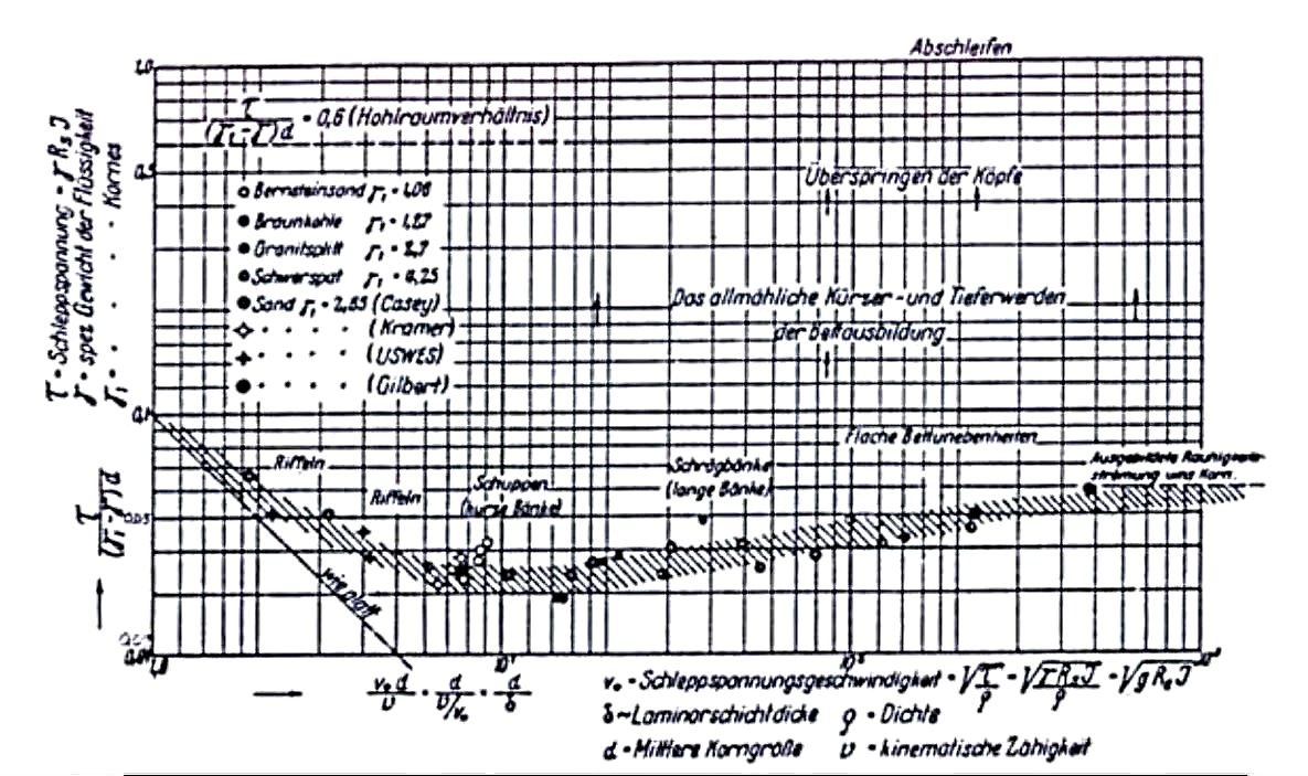
Fìgure 2. Original Shields' diagram. By A. Shields - http://repository.tudelft.nl/assets/uuid:61a19716-a994-4942-9906-f680eb9952d6/Shields.pdf, Public Domain, https://commons.wikimedia.org/w/index.php?curid=36015107
The Shields method can be used to evaluate the stability of sediments into the sea. In fact, given the hydrodynamic forcing acting on the armour unit one can estimate the shear stress τ on the unit itself and then the resulting Shields parameter. If the latter is lower than 0.06 then one may conclude that the unit is stable.
To estimate the shear stress τ acting on the armour unit one has to take into account the forcing originated by waves and currents, which are superimposed each other. Van Rijn (1993) proposed that in such conditions the shear stress is computed as
τ = τcu + τw where τcu and τw are the tangential tensions originated by current and waves, respectively. The following relationships for the computation of the stresses, expressed in N/m2 apply:
τcu = 1/2 ρ fcuu'2
τw = 1/2 ρ fwU'2
with the following meaning of symbols:
- u' is depth-mean current velocity in m/s;
- U' is the velocity of sea water particles due to waves. Before breaking, such velocity is given by the near-bottom peak orbital velocity of fluid particles in m/s, which can be computed according to the linear wave theory by using the relationship:

where Hb, db, T and L0 are significant wave height, water depth, wave period of peak of wave spectrum and significant wave length, respectively. Let us remind that the significant wave height is defined traditionally as the mean wave height (through to crest) of the highest third of the waves. It is also defined as four times the standard deviation of the surface elevation – or equivalently as four times the square root of the zeroth-order moment (area) of the wave spectrum. After breaking, the velocity of particles can be computed through empirical relationships by distinguishing between run-up and run-down along the side of the groin (see, for instance, Schüttrumpf et al. (2001)); - fcu is current related friction factor, which equals about 0.12 (db/ks)0.33, where ks is effective structure side roughness. Its value is about 1.5 d50 for narrow graded stones;
- fw is wave related friction factor, which equals about 0.3 (A/ks)-0.6, where A is near structure peak orbital amplitude.
If the side of the structure is sloped, we indicate with β and β1 the acute angles between the side of the structure and the horizontal plane in the transverse and longitudinal direction, respectively, with respect to the wave direction. Then, we correct τc according to the relationship
τc1=KβKβ1 τc
with the following meaning of symbols:
- Kβ is slope factor in the transverse direction, equal to:


for downsloping and upsloping velocity, respectively; - Kβ1 is slope factor in the longitudinal direction, equal to:
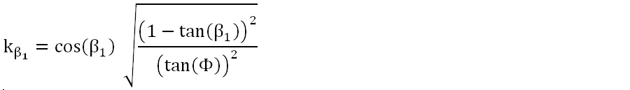 .
.
Small grains are inherently more mobile than large grains. However, on a mixed-grain-size surface they may be trapped in deep pockets between large grains. Likewise, a large grain on a bed of small particles will be stuck in a much smaller pocket than if it were on a bed of grains of the same size. In these cases, small grains can move just as easily as large ones.
Hiding is taken into account in the Shields criteria by correcting the limiting shear stress for incipient mobility. For the case of coastal structures hiding is usually not taken into account, as the armour units are usually narrow graded.
The Shields diagram has been derived basing on several laboratory experiments and therefore already takes into account that the shape of the sediments is not spherical. However, sediments in laboratory experiments usually have a regular shape. If the shape of armour units is highly irregular, for instance when using tetrapods, they might results more stable with respect to what is predicted by the Shields criteria, for the tight interaction between elements. In these case the Shields parameter should be corrected by adopting an equivalent diameter or by laboratory experiments.
Several empirical formulations have been proposed for verifying the stability of armour units when designing coastal structures. They have been mainly derived through laboratory experiments.
Hudson formula (Rock Manual, 2007) dictates the conditions for the stability of rocks/stones under breaking waves at a sloping surface, for waves approaching the structure perpendicularly. It reads as
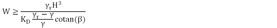
where W is the weight of each armour unit, γr is specific weight of the armour material, β is slope angle of the structure, H is a reference value for wave height which is about 1.27 the significant wave height at the toe of the structure, and KD is an empirical stability coefficient. Several approaches have been proposed for deriving KD, which depends on armour units, type of placement, crest height, type of breaking waves, wave steepness, wave spectrum, permeability of underlayers and many others. The value of KD can be reliably determined only by laboratory experiments on small scale models. KD is usually estimated through the definition of the "critical number" Ncr given by
Ncr = 0.8 (KD cotan(β))1/3 .
Ncr values usually are in the range 1.5 to 3.0 while KD is in the range between 3 and 10. These values typically yield a characteristic diameter for spherical units in the range 0.2 to 0.4 of the significant wave height at the toe of the structure, therefore providing a reference order of magnitude.
Among the methods that are used for estimating Ncr and therefore KD we mention the Van der Meer formula. Further details can be found in Van der Meer (1987) which is available for download here.
Schüttrumpf, H., Troch, P., Walle, B. V. D., Rouck, J. D., & Oumeraci, H. (2001). Prototype run-up velocities at Zeebrugge breakwater. In Coastal Engineering 2000 (pp. 2018-2029).
Van der Meer, J. W. (1987). Stability of breakwater armour layers—design formulae. Coastal engineering, 11(3), 219-239.
van Rijn, L. (2016) Stability design of coastal structures (seadikes, revetments, breakwater and groins, available on-line at www.leovanrijn-sediment.com
Van Rijn, L. C., & Kroon, A. (1993). Sediment transport by currents and waves. In Coastal Engineering 1992 (pp. 2613-2628).
Last modified on March 27, 2021
- 253 views