
The recent concerns on anthropogenic global warming and climate change stimulated an intensive research activity on climate dynamics during the past decades, which emphasised the key role of future climate predictions to devise mitigation and adaptation strategies. These predictions can be produced with alternative and complementary methods than can be possibly integrated in solutions of different complexity, like for instance statistical extrapolation and/or mathematical models of the physics, chemistry, ecology and anthropogenic impact of the climate system.
The history of climate modeling begun with the development of conceptual and very simple models that helped to identify the relevant processes and their connections. For instance, Greek astronomers and geographers understood that the shape of Earth is spherical and connected climate to the inclination of the terrestrial axis. These simple models were followed in the 19th century by mathematical models of energy balance and radiative transfer. Computer simulation models of the atmosphere were first introduced in the 1950s. From the 1990s, when global warming became more and more a concern, increasingly comprehensive models of the entire climate system were developed by integrating an increasing number of physical and chemical processes.
|
2. Climate processes and systems
Climate models are supposed to describe several processes that are linked each others by causal relationships. In fact, climate is governed by a system of physical, chemical, ecological and anthropogenic processes that are linked each other by two-ways connections and feedbacks. One may identify five main subdomains in the climate system:
The cryosphere is the domain of water in solid form, including sea ice, lake ice, river ice, snow cover, glaciers, ice caps, ice sheets, and frozen ground (which includes permafrost). There is a wide overlap between cryosphere and hydrosphere. The cryosphere plays an important role in the Earth’s climate. Snow and ice reflect heat from the sun, therefore contributing to regulate planet’s temperature. Because polar regions are some of the most sensitive to climate shifts, the cryosphere may be one of the first places where scientists are able to identify changes in climate. The hydrosphere includes the mass of water found on, under, and above the surface of a planet. Water in the liquid state covers about 70% of the Earth's surface. About 97% of the liquid water is found in the oceans. Only a small portion of the Earth's water is freshwater, found in rivers, lakes, and groundwater (see Figure 2). The biosphere, also known as the ecosphere, encompasses all ecosystems. It can also be termed the zone of life on Earth and therefore there is a large overlap with other spheres. The biosphere, through photosynthesis, captures solar energy at a rate of around 130 Terawatts/year. It is a system with capacity to self-regulate and is actually close to energetic equilibrium. The technopshere (sometimes also referred as anthroposphere) is that part of the environment that is made or modified by humans for use in human activities and human habitats. The term was first used by nineteenth-century Austrian geologist Eduard Suess. The technosphere is continuously developing and has reached a level of interaction with the climate system that humans never experienced before. In fact, the technosphere is impacting all the other domains above by inducing global feedbacks. These latter compensate impacts therefore contributing to keep the system in equilibrium. However, the connections between the different subdomains are highly nonlinear and therefore the climate system is characterised by thresholds, possible tipping points and several equilibrium states. |
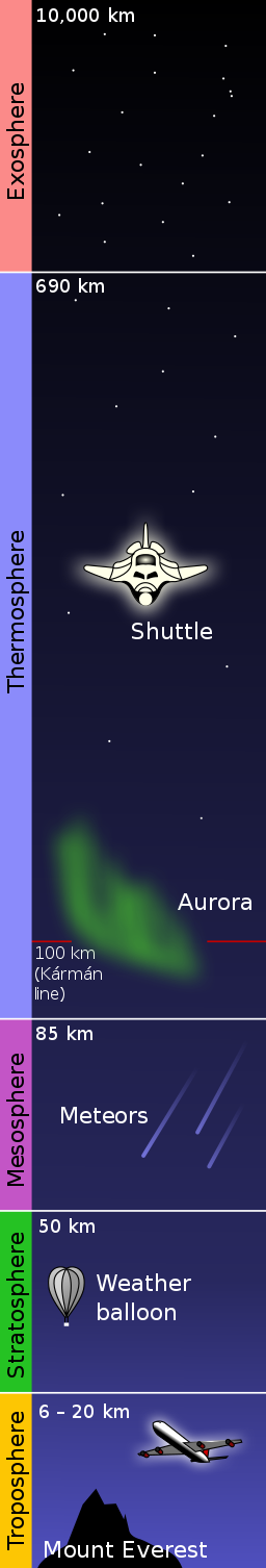 Figure 1. Layers of the atmosphere. Source: NOAA & User:Mysid, Public domain, via Wikimedia Commons Figure 1. Layers of the atmosphere. Source: NOAA & User:Mysid, Public domain, via Wikimedia Commons |
|
The above sudomains are open systems that are tightly related each other, with exchanges of physical quantities like mass, heat, momentum and energy. The climate system is driven by solar energy. Some of it is reflected back into space, while the rest is absorbed by the climate system and re-emitted as heat. Part of the reflected and re-emitted energy is trapped by the Earth's greenhouse effect. This heat dynamics is what determines the temperature of the Earth.
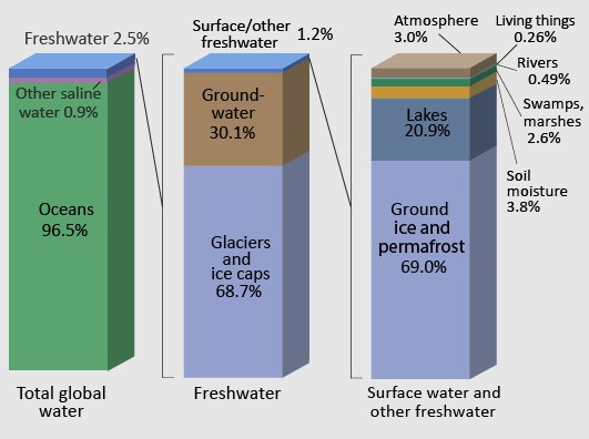
Figure 2. Sketch of water distribution on Earth. By NASA Official website, [1]., Public Domain, https://commons.wikimedia.org/w/index.php?curid=49654959
Earth is heated by sun in an uneven way, as some parts of the Earth receive more energy therefore originating well known temperature differences that the system tends to reduce by transporting heat from the warm tropics to the cool ice zones of the poles. This heat transportation gives rise to ocean currents, wind, evaporation, precipitation, and global weather patterns. In particular, the hydrosphere is intensively connected with the atmosphere through the hydrological cycle, that includes exchanges of water in fluid phase (liquid and gas) and heat through evaporation and precipitation, among other processes. The ocean-atmosphere system also exchanges gases like carbon dioxide, where the ocean acts as a large carbon sink. These interrelationships are not yet fully known and therefore we need to introduce assumptions when building models.
The above systems are characterised by turbulence (figure 3) and may exhibit chaotic behaviours, which imply a high sensitivity to initial and boundary conditions. In terms of predictability, chaotic systems may be predictable in the short term while in the longer term they exhibit uncertainty, that is due to the inflation of the imprecision with which initial and boundary conditions are defined. The time span that the behavior of a chaotic system can be effectively predicted depends on how accurately its current state can be measured, and a time scale depending on the dynamics of the system, called the Lyapunov time. Lack of predictability unavoidably affects environmental models.

Figure 3. Turbulence in the tip vortex from an airplane wing. Studies of the critical point beyond which a system creates turbulence were important for chaos theory. By NASA Langley Research Center (NASA-LaRC), Edited by Fir0002 - This image or video was catalogued by Langley Research Center of the United States National Aeronautics and Space Administration (NASA) under Photo ID: EL-1996-00130 and Alternate ID: L90-5919., Public Domain, https://commons.wikimedia.org/w/index.php?curid=494937
Climate models reproduce the functioning of climate with the purpose of gaining a better understanding of how this complex systems works by testing theories and solutions. The second purpose of climate models is to reproduce the distribution in space and time of key variables of the atmospheric system, such as temperature, wind, rainfall and so forth. These variables are affected by significant spatial heterogeneity - with different behaviours depending on the specific variable - and are also quickly varying in time.
Global climate models are mathematical representation of the climate system's dynamics. They range from very simplified mathematical representation, like the so-called box models, to complex emulations of the whole system that apply a set of physical equations at local scale, like the General Circulation Models (GCM). GCMs are frequently applied in climate studies to predict the future climate depending on assigned initial and boundary conditions and assigned input variables and parameters. GCMs have developed rapidly over recent decades in response to increasing interest in climate modeling, major advances in computing power and better understanding of how the climate system works.
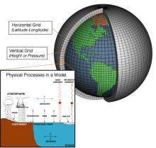
GCMs equations describe the evolution in space and time of relevant atmospheric processes, by introducing hypotheses and simplifications that allow a tractable representation of the climate system. In view of their heterogeneity such processes are described at local scale by discretising the atmosphere into a 3-dimensional grid (figure 4). Any grid box is assumed to be a representative elementary volume over which a measurement of the relevant variables is assumed to be representative of the corresponding volume value. The boxes have variable dimension, with increasing computational demand for decreasing box size. Modern models have box size, projected over the land, varying from 100 square kilometers for detailed models to 600 square kilometers for coarser representations. Click here to see an animation presenting the evolution of grid sizes during the progressive development of models. The results of processes modeled in each cell are passed to neighboring cells to model the exchange of quantities over space and time.
Candidates equations to describe the system at local scale are conservation laws which state that a particular measurable property of an isolated physical system within a reference region of space does not change as the system evolves over time. Conserved physical quantities may be, for instance, energy, momentum, mass, and water vapor. A local conservation law is usually expressed as a continuity equation. It is a partial differential equation which gives a relation between the amount of the quantity and its transport. In detail, the continuity equations states that the amount of the conserved quantity within a volume can only change by the amount of the quantity which flows in or out of the volume. The fact that the equation describes “change” justifies its differential form. To simulate the value of the variables we need to sum their changes over the grid and over the infinitesimal time steps, therefore performing an integration over space and time. Integration requires the knowledge of the initial and boundary conditions, which dictate the values to be assumed by the variables at a given time and the boundary of their spatial domain.
Therefore, climate models essentially describe how energy and materials propagate through the climate system, which includes atmosphere, land and oceans. Developing and running a GCMs requires identifying and quantifying Earth system processes, representing them with the above equations, setting variables to represent initial conditions and subsequent changes in climate forcing, and repeatedly solving the equations using powerful supercomputers.
The relevant computational resources required by GCMs are only available at a limited number of computational centers around the world. These required resources are continuously increasing as models evolves. Early generations models relied on simplifying assumptions and solutions which made the coupling of ocean and atmosphere particularly difficult. Recent models solved these problems and also incorporate aerosols and vegetation dynamics and atmospheric chemistry. They also better represent the carbon cycle and a range of CO2 emission scenarios is now employed based on assumptions on the socioeconomic evolution of the global community.
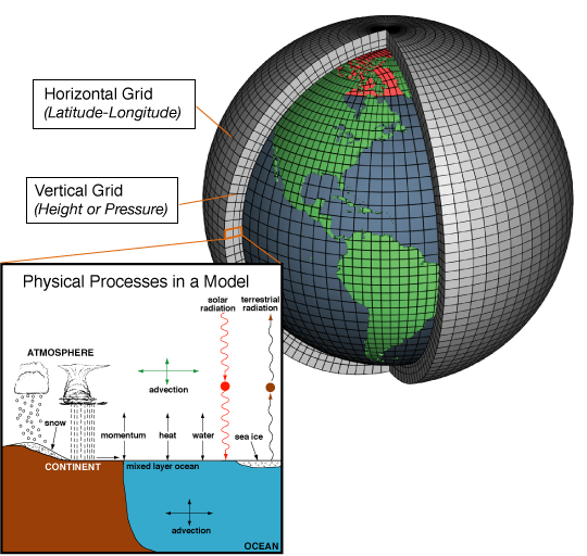
Figure 4. Grid representation of the climate system by GCMs. Processes that are reproduced include physical and chemical phenomena. Image source: NOAA.
Input data for climate models are the driving forces for the climate itself, which may be collected through observation and future predictions. Solar forcing is one of the main inputs, which is quantified by estimating current and future solar activity and how much of the solar energy is trapped by the atmosphere and absorbed by Earth. Another relevant driving force, which is also related to the human impact, is the concentration of greenhouse gases like CO2, methane (CH4), nitrous oxides (N2O) and halocarbons – as well as aerosols that are emitted when burning fossil fuels. Aerosols reflect incoming sunlight and influence cloud formation. Today, most model projections use one or more of the “Representative Concentration Pathways” (RCPs) of greenhouse gases, which provide plausible descriptions of the future, based on socio-economic scenarios of how global society grows and develops. See here for more information and see Section 5 below for a more extended discussion.
Output data from climate models depict a picture of the Earth’s climate, through thousands of different variables across hourly, daily and monthly timeframes. These variables include temperatures and humidity of different layers of the atmosphere from the surface to the upper stratosphere, as well as temperatures, salinity and acidity (pH) of the oceans from the surface down to the sea floor. Models also produce estimates of snowfall, rainfall, snow cover and the extent of glaciers, ice sheets and sea ice. They generate wind speed, strength and direction, as well as climate features, such as the jet stream and ocean currents. A full list of outputs from the climate models being run for the next IPCC report are available from the Coupled Model Intercomparison Project (CMIP) by the World Climate Research Programme. It is a cooperative framework to better understand past, present and future climate changes arising from natural, unforced variability or in response to changes in radiative forcing in a multi-model context. CMIP has been articulated in several phases. The current one is the sixth and is named CMIP6, while the most recently completed phase of the project (2010-2014) is CMIP5. The IPCC Fifth Assessment Report summarizes information of CMIP5 experiments.
A key feature of GCMs output is the time step, which typically is 30 minutes and is influential also on simulation performance. For instance, the partitioning between precipitation determined by large-scale dynamics versus cumulus parameterization is sensitive to model time step, with implications for rainfall extremes (see Yu and Pritchard, 2015). In fact, a finer time scale implies that short time variability in precipitation is better described, but it is not yet clear whether extremes that result from subhourly events are well described. For this reason output of climate models, for certain variables, are presented in terms of longer term statistics. These statistics are often downscaled in space and time using limited area models such as the regional climate models (see the overview by Giorgi (2019)) or stochastic weather generators. The latter may also allow to generate future point rainfall. Both regional climate models and weather generators can be initialised by using statistics generated by GCM.
Weather generators may allow to overcome the problem of the poor fit of GCM models of the statistics of precipitation extremes. For instance, average values for precipitation produced over a given time step may be used to condition the corresponding statistics of the weather generator, while statistics of the extremes at shorter time step may be constrained by using historical data and stochastic projections.
An interesting approach is stochastic simulation, which combines statistical and physically based modelling. Accordingly, the projections of future climate are obtained through a statistical approach which is obtained by projecting into the future the statistics of the past climate. These statistics can be corrected by taking into account the predictions of climate models when appropriate. An interesting example of this technique was recently provided by Kiem et al. (2021). From their abstract one reads:
" In this study, we develop an approach for stochastically generating future seasonal (monthly to annual) hydroclimatic conditions at multiple sites for water supply security assessment that capitalizes on an Australia‐wide relationship between annual average daily maximum temperature and annual rain (and flow). This approach is practical as it (i) avoids the extra time and additional uncertainties introduced by downscaling and bias correction of climate model produced rainfall information and (ii) takes advantage of the fact that climate model projections for temperature change are more realistic than climate model projections for rainfall."
Whatever solution is applied to downscale climate model output in space and time, one needs to take into account that a finer resolution does not necessarily imply improved performances. For instance, the "Guidance: Caveats and llimitations" of the United Kingdom Climate Programme 2018 (UKCP18) says:
Global climate models provide greater confidence for long-term climate averages than extreme events or time series of daily or sub-daily values. All climate models exhibit systematic differences between model results and observations and you need to consider whether to modify the datasets to correct for these. This is called bias-correction and is a popular approach used by many researchers and climate data users. Take care when applying these methods, as debatable assumptionsf are often required and bias-correction may not be appropriate.
and
Downscaling – the process of generating model data at higher spatial and/or temporal resolution – adds detail but also increases the level of uncertainty. The additional information content can be useful for applications that wish to understand how small-scale features such as mountains and coastlines or land surface features may influence the local climate and their system of interest. However, finer model spatial resolution does not necessarily provide greater confidence in modelling the climate system unless it has been shown to give a better representation of the underlying physical processes.
Therefore, a through appraisal of model performances is needed before using data for technical applications.
We mentioned that climate models are much computationally intensive. They require powerful supercomputers and considerable human and economic resources. Moreover, their run may require a lot of time.
To make the simulation easier and faster, we have the option of using simpler models – called “emulators”. These may produce simulations with a relatively limited use of resources. Instead of simulating the whole set of climatic variables, emulators may be limited to selected climatic features like, for instance, sea level rise, regional climate change and so forth.
Emulators have an history that is about as long as climate models. The IPCC has used emulators throughout its history. Their role was less important for the development of the fifth assessment report (AR5). For the recently released AR6 WG1 report, and the related Climate Model Intercomparison Project 6 (CMIP6), emulators have returned to a more prominent role. In fact, the simulations by full climate models that have been produced for AR6 resulted in very high levels of projected future warming in several models, that lied outside the expected range. Using emulators that have been calibrated with observationally constrained results brought down the high end-of-century projected future warming by some models.
A climate model emulator may count several different parameters that control different features of the climate system, such as the warming and cooling impact of air pollution, how heat diffuses in the ocean, and the response of land and ocean carbon sinks to global warming. By simultaneously varying parameters, emulators can be "tuned”. For example, we know that the airborne fraction of CO2 – the proportion of CO2 emitted that remains in the atmosphere following emission – depends on the strength of land and ocean carbon sinks, which in turn are dependent on temperature and total carbon stored in those sinks. We might make an educated guess at the functional form of this relationship, and then fit this relationship from dedicated model experiments (for more details see CarbonBrief.org).
Unlike full models, emulators can produce a climate projection in a fraction of a second on a desktop computer. This means that emulators can be run hundreds, thousands or even millions of times for a single emissions scenario with different parameter values. This is important in order to span the range of uncertainty around future climate projections. Not all parameter combinations will produce realistic climate projections. One indicator of “realism” is whether an emulator can reproduce a good representation of the historically observed climate change.
As we can run very large sets of emulator projections, we can reject simulations that do not correspond well to historical observations. Given that data are not perfect themselves, we can build in the observational uncertainty around these best estimate values, too. This results in a much smaller, constrained set of projections than one started with, but one in which more confidence can be given.
For instance, Figure 5 shows how global warming in CMIP6 models (red lines) compare to historical temperature observations (blue). Using an emulator that is calibrated to CMIP6 results, a range of projections can be produced (light grey). However, when we introduce observational constraints, the range of uncertainty is narrowed (dark grey) by eliminating some of the more implausible projections, producing a best estimate future projection (black) that closely follows the observed warming. This method corrects for some of the systematic biases in CMIP6 models, for example a tendency to underpredict the warming in the late 20th Century (Smith, 2021)
.
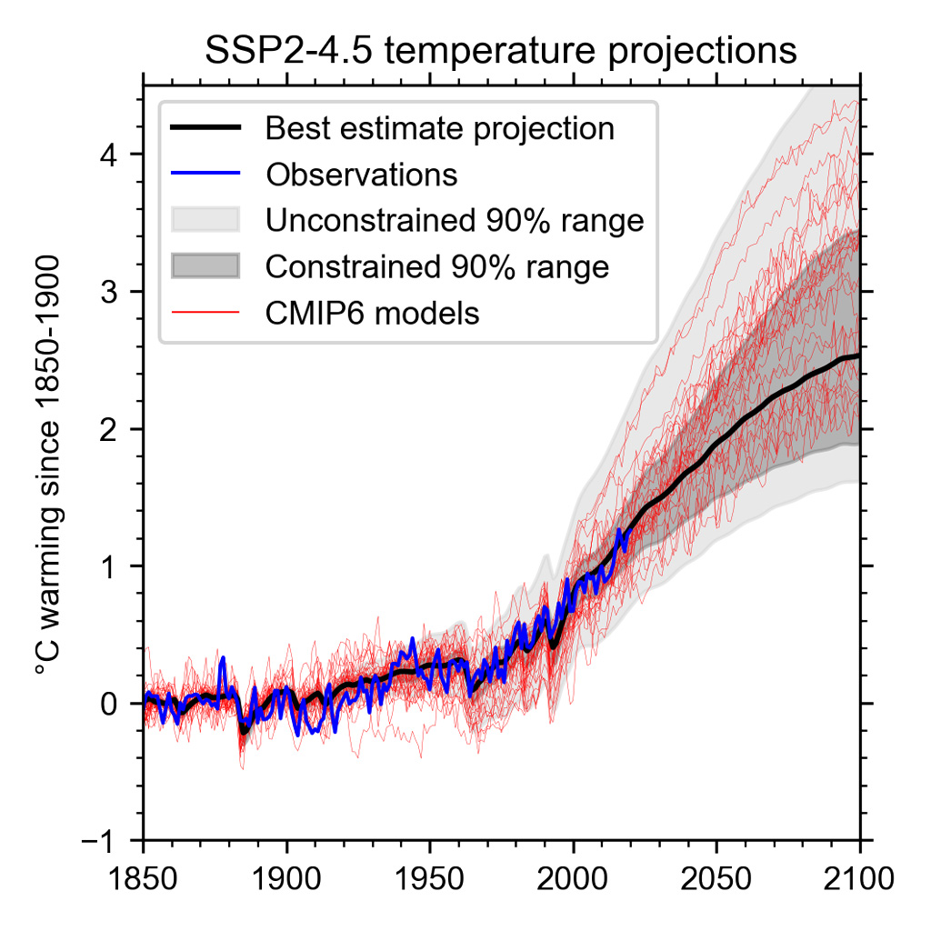
Figure 5. Demonstration of constraining a large ensemble of prior runs following the SSP2-4.5 emissions pathway (light grey) into a smaller ensemble of runs that satisfy assessed ranges of historical warming, climate sensitivity, ocean heat content change and CO2 (dark grey), with best estimate in black. Historical observed warming is shown in blue and individual CMIP6 model runs are shown in red. Credit: Chris Smith through CarbonBrief.org.
One of the many strengths of emulators is that they can be used to run climate scenarios not analysed by full models. One meaningful example is the attribution of present-day warming to emissions of different gases and aerosols (Figure 6). The bars indicate emissions that have an overall warming (red) or cooling (blue) effect, with the total human-caused impact shown in grey.
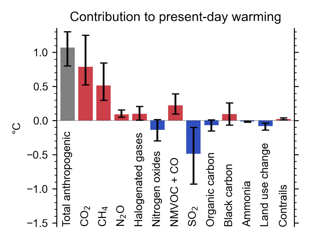
Figure 6. The contribution to present-day warming from emissions, determined using an emulator. Adapted from IPCC AR6 WG1 (2021) Summary for Policymakers Figure 2c by Chris Smith through Carbonbrief.org.
Being able to run a large number of simulations means that indications can be derived on the uncertainty in the temperature response to each forcing.
A very simple example of climate model which consider the whole system an a homogeneous entity is based on the concept of radiative equilibrium, which is described by the equation
(1 - a)Sπr2 = 4πr2εσT4
where:
- S is the solar constant – the incoming solar radiation per unit area—about 1367 W·m−2;
- a is the Earth's average albedo, which is about 0.3;
- r is the radius of Earth, which is about 6.371×10⁶m;
- σ is the Stefan-Boltzmann constant, that is about 5.67×10⁻⁸ J·K−4·m−2·s−1;
- ε is the effective emissivity of earth, about 0.612
Solving for the temperature one obtains:
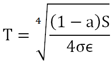
The above equation, which yields an apparent effective average earth temperature of 15 °C, illustrates the effect on average earth temperature of changes in solar constant or change of albedo or effective earth emissivity.
Examples of GCM models are, for instance, those considered by the CMIP project. An introduction to climate models in the contect of CMIP is given by this video. GCM models considered in CMIP are, for instance, the < href=http://www.glisaclimate.org/node/2239 target=_blank>CSIRO-Mk3-6-0 by the Commonwealth Scientific and Industrial Research Organization/Queensland Climate Change Centre of Excellence, the CanESM2 by the Canadian Centre for Climate Modelling and Analysis, and the HadGEM3 by the Met Office Hadley Centre.
An important input value for climate models is the future concentration of atmospheric CO2. In 2000, the Intergovernmental Panel on Climate Change (IPCC) published the "Special Report on Emissions Scenarios" (SRES), describing four scenario categories corresponding to a range of possible future conditions. Each scenario was based on assumptions on the socioeconomic drivers of greenhouse gas and aerosol emissions and the levels to which those emissions would progress during the 21st century.
In 2013, climate scientists defined a new set of scenarios that focused on the level of greenhouse gases in the atmosphere in 2100. These scenarios are known as Representative Concentration Pathways or RCPs. Each RCP indicates the amount of climate forcing, expressed in Watts per square meter, that would result from greenhouse gases in the atmosphere in 2100. Therefore, there is a key change from the previous approach in that the RCPs focus on concentrations of greenhouse gases, not greenhouse gas inputs, by ignoring the carbon cycle. The reason for such a decision is that large uncertainty is implied by the modelling of terrestrial carbon cycle, which is influenced by both climate change and land use change. The rate and trajectory of the forcing is the pathway. The RCPs scenarios are:
- RCP 1.9: a pathway intended to limit global warming to below 1.5 °C,which is the aspirational goal of the Paris Agreement.
- RCP 2.6: a very stringent pathway requiring, among the others, that carbon dioxide (CO2) emissions start declining by 2020 and go to zero by 2100.
- RCP 3.4: an intermediate pathway between RCP2.6 and the less stringent mitigation efforts associated with RCP4.5.
- RCP 4.5: an intermediate scenario. Emissions in RCP 4.5 peak around 2040, then decline.
- RCP 6: according to this scenario, emissions peak around 2080, then decline.
- RCP 7: a baseline outcome rather than a mitigation target.
- RCP 8.5: it is also called the "business as usual scenario", where emissions continue to rise throughout the 21st century. It is considered an unlikely but still possible scenario.
Figure 7 shows a graph of the progress of emission scenarios along time (from CarbonBrief.org). Two estimated emission pathways are represented for each scenario: the RCPs considered by the Coupled Model Intercomparison Project 5 (CMIP5, dashed lines) and their new CMIP6 SSPs (solid lines).
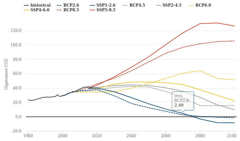
Figure 7. Future emissions scenarios featured in the Coupled Model Intercomparison Project 5 (CMIP5, dashed lines) and their new CMIP6 counterparts (solid lines).
Recently, there have been several discussion on the likelihood of RCP 8.5. For more information please see, for example, Hausfather and Peters (2020) and Schwalm et al. (2020).
Uncertainty assessment is a core topic for all the disciplines involved in environmental modelling. Methods and terminology that are applied in sister disciplines differ a lot. For instance, uncertainty is assessed in climate with a much different perspective with respect, for instance, to hydrology and economics. This is the result of the fact that different level of uncertainty can be tolerated in different applications. What is a unbearable uncertainty for engineering applications may be tolerated in economics and viceversa.
Climate modelers are most concerned about three types of uncertainty:
- forcing uncertainty,
- model uncertainty and
- uncertainty over initial conditions.
Forcing uncertainty mainly arises from emission scenarios that describe future emissions and human activity. These are predictions based on fundamentally different assumptions about future human socio-economic development and political strategies, which are of course very difficult to predict. In fact, they come from complex and often chaotic economic and socio-political processes, that are also influenced by natural or human induced events. The most relevant recent example is the occurrence of COVID-19 which caused a global reduction of CO2 emissions. Forcing uncertainty is probably the largest uncertainty in future climate projections.
Model uncertainty, also termed model structural uncertainty, reflects the fact that models are an approximation of reality, and therefore would be affected by uncertainty even if perfect input variables and initial conditions were used. This is due to the fact that we do not yet have the "correct" climate model available. Relevant uncertainties are due, for instance, to subgrid parameterisation and still imperfect representation of the feedbacks among multiple processes.
Regarding initial conditions, they are relevant to uncertainty as the models exhibit chaotic behaviours (see above). The realization that perfectly deterministic systems may exhibit unpredictable behavior (Lorenz, 1963) is considered one of the greatest scientific discoveries of the twentieth century. In fact, for nonlinear dynamical systems such as atmosphere, ocean and land waters, any uncertainty in the initial state - however small - may grow sufficiently rapidly in time to make impossible to predict the state of the system beyond some finite time horizon.
Climate models are tested by reproducing data that were observed in the past. Testing a model by comparing observed and simulated data is a classical procedure in environmental modelling, which is however applied with different protocols in the various disciplines. For instance, comparison may be carried out by comparing data or their statistics (see figure 5). Model testing includes adjusting model equations and their parameters to improve the fit. Models that do not reproduce well historical climate scenario can be adjusted by correcting their simulation to match selected statistics of the observed climate. One of these procedure is bias correction, which however corrects only selected statistics of the data.
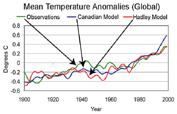
Figure 8. Trends of global temperature from observations, the United Kingdom’s Hadley Centre Global Climate Model, and the Canadian Climate Center’s Global Climate Model from 1900 to 2000. Trends have been smoothed to remove year-to-year high frequency variations. Public Domain, https://commons.wikimedia.org/w/index.php?curid=1104732
Uncertainty of climate model simulation is often evaluated by ensemble prediction. Instead of making a single prediction by using a single model and a single input information and parameter values, a set (or ensemble) of predictions is produced, by using several models and/or several input data and initial and boundary conditions. This set of predictions is assumed to give an indication of the range of possible future climates. The range of the predictions is expected to encompass two sources of uncertainty that were described above: (1) the errors introduced by the use of imperfect input data and initial conditions, which is amplified by the chaotic nature of the atmosphere; and (2) errors related to model structural uncertainty. Actually, the latter uncertainty is only partially accounted for by ensemble prediction, as the true value of the future climate is not necessarily encompassed by the range of the predictions. An interesting note in this respect is offered by Brown et al. (2012):
A problem with this approach is that GCM projections are relatively poor scenario generators. They describe a “lower bound on the maximum range of uncertainty” (Stainforth et al., 2007). Even a large multimodel ensemble provides relatively few samples in a typical analysis relative to the size possible through stochastically generated risk analysis. Larger ensembles are becoming available, such as via the climate prediction.net experiment (Stainforth et al., 2004) but still face issues of biases that may preclude the discovery of plausible climate risks.
The result from ensemble modelling is often referred to a “multi-model ensemble”. The outcomes from ensembles may be averaged to obtain a best estimate that may be needed for practical applications. In such a case, it is important to recall that variability around the mean may be poorly estimated from the ensemble. For example, if an economist was to estimate crop losses due to temperature changes over time and the loss function is nonlinear and concave, the losses calculated using temperatures from a multi-model ensemble may be incorrect if the variance in temperatures around the mean is poorly estimated or the distribution of ensembles around their mean is asymmetric.
Figure 9 shows simulations by several climate models under an assigned future emission scenario (SRES-A2).
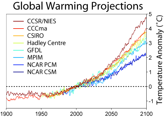
Figure 9. Climate model predictions for global warming under a given (SRES-A2) emissions scenario relative to global average temperatures in 2000.
Padrón et al. (2018) noted that projections of future water availability vary substantially across different models and found that such disagreement can be reduced by placing more confidence on models that more accurately reproduce observed rainfall amounts. In particular, they showed that previous projections of very extreme future changes in water availability are less likely to occur. Moon et al. (2018) investigated how well current generation models represent drought persistence over the twentieth century and the recent past. They highlighted that the considered models tend to underestimate drought persistence at monthly and annual time scales.
Moreover, downscaling methods such as regional climate models or weather generators introduced additional uncertainty which should be properly considered (see also the previous section 4).
The above uncertainties are the subject of intensive ongoing work by the scientific community. At the present stage, however, what-if scenarios produced by climate model are useful to provide projections of future climate statistics, provided their uncertainty is duly taken into account.
The impact of climate change can be contrasted through mitigation and adaptation strategies. Climate change mitigation consists of actions to limit the magnitude or rate of climate change. Actions primarily consists of reductions in human emissions of greenhouse gases. Mitigation may also be achieved by increasing the capacity of carbon sinks, e.g., through reforestation or other methods.
Emission reductions have been discussed in several international conferences like the United Nations Framework Convention on Climate Change, which issued the Kyoto Protocol and the United Nations Climate Change conference (COP). The target is to reach international agreements that bind countries to emission reduction targets. In 2010, Parties to the UNFCCC agreed that future global warming should be limited to below 2.0 °C relative to the pre-industrial level. With the Paris Agreement of 2015 this was confirmed, but was revised with a new target laying down "parties will do the best" to achieve warming below 1.5 °C. Current level of warming is recognized around 0.8 °C.
Emission reduction has several impacts on economy and politics and therefore reaching an international consensus is not an easy task. The problem is also complicated by the uncertainty related to the effectiveness of reducing emissions. While the target certainly implies relevant benefits, including reduction of air pollution, it would not lead to significant mitigation of climate change if the latter was mainly due to natural variability. Given the high societal cost associated to emission reduction, the above question is highly relevant to sustainable development.
Climate change adaptation is a response to climate change aiming at reducing the vulnerability of social and biological systems to relatively sudden change and thus offset the effects of global warming. While climate change mitigation is a typical top-down approach, climate change adaptation is an example of the so-called "bottom-up" approach to sustainability, which is discussed here. Climate change adaptation focuses on resilience and sustainability of current societal systems and therefore it is based on "people" rather than politics. Also, climate change adaptation involves actions to be taken at several spatial scales and therefore distributes the responsibility for social security over local, regional and country administrations. Adaptation is especially important in developing countries since those countries have a reduced capacity and potential for humans to adapt (called adaptive capacity).
Scheraga and Grambsch (1998) identify 9 fundamental principles to be considered when designing adaptation policy:
- The effects of climate change vary by region;
- The effects of climate change may vary across demographic groups;
- Climate change poses both risks and opportunities;
- The effects of climate change must be considered in the context of multiple stressors and factors, which may be as important to the design of adaptive responses as the sensitivity of the change;
- Adaptation comes at a cost;
- Adaptive responses vary in effectiveness, as demonstrated by current efforts to cope with climate variability;
- The systemic nature of climate impacts complicates the development of adaptation policy;
- Maladaptation can result in negative effects that are as serious as the climate-induced effects that are being avoided;
- Many opportunities for adaptation make sense whether or not the effects of climate change are realized.
More details can be found in my lecture Climate change and water cycle.
Comprehensive technical guidelines for designing engineering infrastructures for climate change adaptation are still lacking. There is an extended literature discussing non-stationarity and its implications (see also Montanari and Koutsoyiannis, 2014) but it is still not clear if non-stationary models can provide reliable design variables and how non-stationary models should be applied in view of the information provided by climate models.
The literature presented several applications where the impact of climate change is estimated through the application of scenario analysis according to the so-called top down approach: simulations by climate models are used as input variables to assigned environmental models which in turn are tasked to produce the required design variables to address the vulnerability of the given system. The problem with this approach is that using a cascade of models implies a cascade of uncertainties which interact in a non-linear fashion and may therefore produce an inflation of uncertainty itself. As such, the obtained design variables may be not precise enough to support technical applications. One should bear in mind that the uncertainty that may be tolerated for future climate scenario may be too large for technical design, for which ethical and legal responsibilities require that the estimation of design variables is rigorously carried out. To give an example, there is variation in climate across the discrete grid cells of climate models. For example, if one uses a climate model providing output at a monthly time scale, temperatures within the month and among all locations in the grid cell are considered constant, which is of course not the case. The size of grid cell may be small from the perspective of the global climate, but not from the perspective of human systems. This becomes especially relevant if the underlying topography is not flat but mountainous or is located near the ocean. In the absence of an appropriate downscaled dataset for the region and time step of interest, the most common practice is to adopt a downscaling model which may also be used to correct the bias of climate simulations with respect to observed data. If this approach is used, however, only selected statistics will be downscaled and corrected and therefore it is important to estimate the resulting uncertainty. In summary, one should be very careful when simply using GCM output as a direct forecast of future climate in impact estimation relative to a weather station-based baseline climate, even if the forcing scenario on which the simulation is based was accurate (Auffhammer et al., 2011).
If scenario analysis is used, uncertainty of the results should be estimated with a rigorous approach that cannot be limited to an estimation of a scenario envelope. In fact, those envelopes general do not fully account for model structural uncertainty, which is a relevant source of error for both climate and environmental models (see Montanari et al., 2011, for a discussion on model structural uncertainty). On the other hand, if uncertainty is rigorously estimated for a cascade of models the resulting uncertainty envelopes (confidence intervals) often result very large therefore leading to economically and environmentally unsustainable solutions.
With the awareness of the above limitations, the literature recently discussed solutions to support decision making when dealing with the technical design of climate change adaptation solutions. Relevant examples are robust decision making and decision scaling.
Robust Decision Making (RDM) characterizes uncertainty with multiple views of the future given the available knowledge of uncertainty. These multiple views are created by just looking at their possibility, without necessarily taking into account their probability. Then, robustness with respect to those multiple views, rather than optimality, is adopted as a criterion to assess alternative policies. Several different approaches can be followed to seek robustness. These may include, for instance, trading a small amount of optimum performance for less sensitivity to broken assumptions, or performance comparison over a wide range of plausible scenarios. Finally, a vulnerability-and-response-option analysis framework is used to identify robust strategies that minimize the regret that may occur over the different future scenarios. This structuring of the decision problem is a key feature of RDM which has been used in several climate adaptation studies (see, for instance, Bhave et al., 2016 and Daron (2015)).
Details on RDM are given here and briefly summarized here below.
- Step 1: identification of future scenarios, systems models and metrics to evaluate success. The first step in RDM is articulated by a joint work among stakeholders, planners, and decision makers. They sit together to identify possible future scenarios, without caring of their probability in this stage. Therefore, uniform sampling may be used rather than basing on a prior distribution, in order to make sure that all possibilities are explored. Metrics to describe how well future goals would be met are also agreed upon. Metrics can be, for instance, water demands or water supplied, or unmet demand. Metrics can also include indexes such as reliability (e.g. the percentage of years in which the system does not fail). Environmental and/or financial metrics can also be considered such as minimum in-stream flows and costs of service provision. Furthermore, in this step candidate strategies for reaching the goals are identified, such as investments or programs. They also agree on the models that will be used to determine future performances of the system.
- Step 2: evaluation of system performances. In this step, which is termed as "experimental design", the performances of the alternative strategies are evaluated with respect to the possible future scenarios, by estimating the related metrics of success. This step is typically analytical.
- Step 3: vulnerability assessment. Stakeholders and decision makers work together to analyse the results from step 2 to identify the vulnerabilities associated to each strategy. The results from the simulations in Step 2 are first evaluated to determine in which futures the management strategy or strategies do not meet the management targets. Next, a scenario discovery leads stakeholders and decision makers to jointly define a small number of scenarios to which the strategy is vulnerable. The information about vulnerability can help define new management options that can be used to test strategies more robust to those vulnerabilities. Furthermore, they identify tradeoffs among different strategies. The vulnerability analysis helps decision makers recognize those combinations of uncertainties that require their attention and those that can instead be ignored. Visual inspection or more sophisticated statistical analyses can be used depending on the problem and audience.
- Step 4: adaptation options to address vulnerabilities. The information on system's vulnerability can then be used to identify the most robust adaptation option. Moreover, suggestions to improve the considered options can also be gained from step 3. For instance, adaptive strategies can be considered, that can evolve over time depending on the observed conditions. Interactive visualizations may be used to help decision makers and stakeholders understand the tradeoffs in terms of how alternative strategies perform in reducing vulnerabilities. This information is often paired with additional information about costs and other implications of strategies.
- Step 5: risk management. At this stage decision makers and stakeholders can bring in their assumptions regarding the likelihoods of the future scenarios and the related vulnerable conditions. For example, if the vulnerable conditions are deemed very unlikely, then the reduction in the corresponding vulnerabilities may not be worth the cost or effort. Conversely, the vulnerable conditions identified may be viewed as plausible or very likely, providing support to a strategy designed to reduce these vulnerabilities. Based on this tradeoff analysis, decision makers may finally decide on a robust strategy.
RDM characterizes uncertainty in the context of a particular decision. That is, the method identifies those combinations of uncertainties most important to the choice among alternative options and describes the set of beliefs about the uncertain state of the world that are consistent with choosing one option over another. This ordering provides cognitive benefits in decision support applications, allowing stakeholders to understand the key assumptions underlying alternative options before committing themselves to believing those assumptions.
RDM reverses the order of traditional decision analysis by conducting an iterative process based on a vulnerability-and-response-option rather than a predict-then-act decision framework, which is adaptation based on a single projected future. This is known as a bottom-up analysis and differs from the top-down method that is also widely utilised in decision making (Blöschl et al., 2013).
Decision-scaling (DS) is another bottom-up analysis approach to decision making. It has been introduced in the context of climate change adaptation (Brown et al., 2012). The term "decision scaling" refers to the use of a decision analytic framework to investigate the appropriate downscaling of climate information that is needed to best inform the decision at hand. Here downscaling refers to the identification of the relevant climatic information from the large ensemble of simulations provided by Global Circulation Models (GCMs). DS differs from current methodologies by utilizing the climate information in the latter stages of the process within a decision space to guide preferences among choices.
The analytical heart of DS a kind of “stress test” to identify the factors or combinations of factors that cause the considered system to fail. Thus, in the first step of the analysis vulnerabilities are identified. These vulnerabilities can be defined in terms of those external factors and the thresholds at which they become problematic. The purpose is to identify the scenarios that are relevant to the considered decision which serve as the basis for any necessary scientific investigation.
In the second step of the decision making process, future projections of climate are then used to characterise the relative likelihood or plausibility of those conditions occurring. By using climate projections only in the second step of the analysis, the initial findings are not diluted by the uncertainties inherent in the projections. In the third step of the analysis strategies can be planned to minimize the risk of the system.
The result is a detected ‘vulnerability domain’ of key concerns that the planner or decision maker can utilise to isolate the key climate change projections to strengthen the respective system against, which differs from the bottom-up analysis featured in RDM (see figure 8).This setup marks DS primarily as a risk assessment tool with limited features developed for overall risk management.
The workflow of DS is compared with the one of RDM in figure 10, where the workflow of the traditional top-down approach is also depicted.
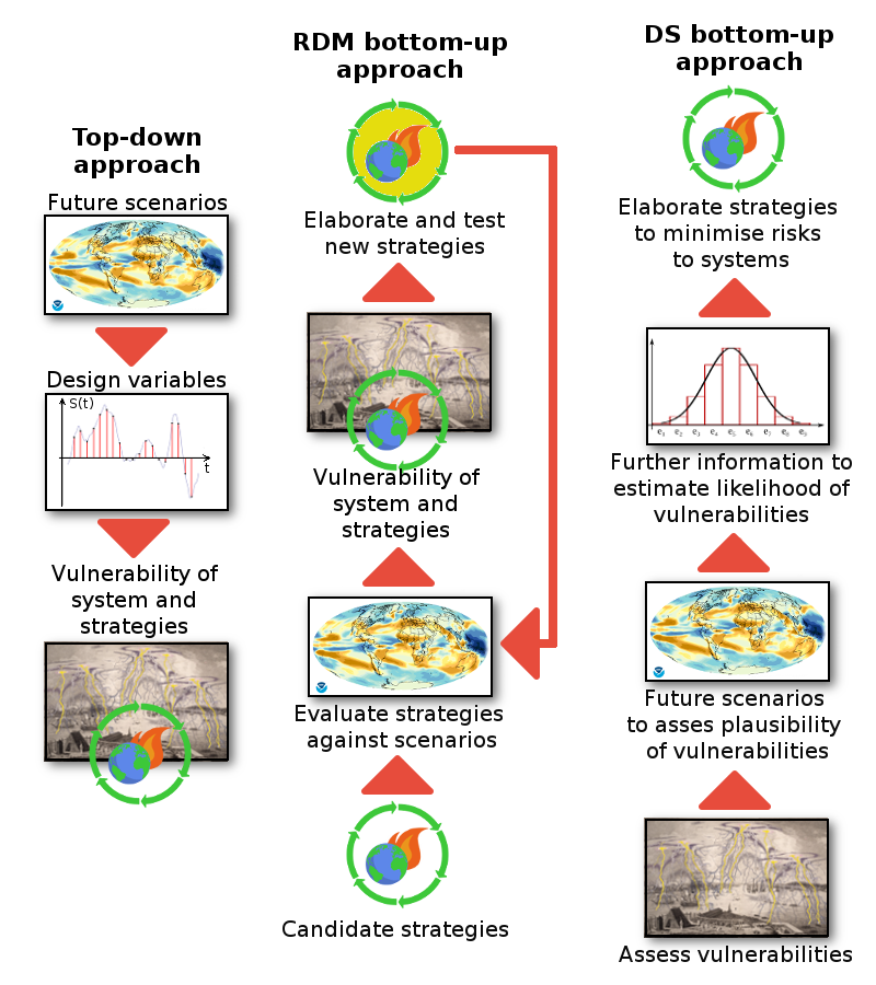
Figure 10. Top-down decision approach versus DS and RDM bottom-up approaches – adapted from Roach (2016), Brown et al. (2012), Hall et al. (2012) and Lempert and Groves (2010). Images are taken from the following sources: NOAA Geophysical Fluid Dynamics Laboratory (GFDL) [Public domain], Mike Toews - Own work, CC BY-SA 3.0, https://commons.wikimedia.org/w/index.php?curid=15592558, James Mason [Public domain], Dan Perry [CC BY 3.0 (https://creativecommons.org/licenses/by/3.0)], Tommaso.sansone91 - Own work, CC0, https://commons.wikimedia.org/w/index.php?curid=77398870, Svjo - Own work, CC BY-SA 3.0, https://commons.wikimedia.org/w/index.php?curid=20327097.
Finally, one may consider to compare the simulations of future climate given by climate models with those provided by stochastic simulation, which may be obtained by using stationary and non-stationary models. Stochastic simulation is based on the assumption that the considered design variable is a random variable. This association is particularly useful in the presence of uncertainty. In fact, randomness is directly associated to the uncertain value of the considered variable. Stochastic simulation is a technique to trace the uncertain evolution of variables that can change stochastically (randomly) with certain probabilities.
The rationale behind stochastic simulation is to characterise the actual dynamics of relevant systems through an inductive approach, namely, through data driven techniques. Recent developments (Montanari and Koutsoyiannis, 2012) elaborated a framework that allows one to take into account physically based knowledge in inductive reasoning. That is, the available knowledge of the system is used to condition stochastic assessment and simulation.
Stochastic simulation is applied in classical water resources management by creating several future scenarios that are obtained by simulating observations that have not been observed, but are equally likely with respect to observed values. Namely, the simulated time series have the same statistics of historical data. These steps are repeated until a sufficient amount of data is gathered. The distribution of the outputs shows the most probable estimates as well as a frame of expectations regarding what ranges of values the variables are more or less likely to fall in.
In the presence of climate change, past and current system conditions may not be representative of what will occur in the future. However, they are still representative of system's behaviors and therefore their assessment is an essential step for deciphering how the system itself may react to change. Therefore, a possible opportunity for estimating design variables under changing condition may be articulated into three main steps which may be identified with the term "stochastic change simulation":
- Assessment of current system's conditions through stochastic analysis;
- Estimation of the impact of change on system's relevant statistics;
- Generation of future scenarios under change through stochastic simulation.
The first step above is carried out by using classical statistical analysis. The second step may be resolved by expert knowledge and/or assessing the output of climate models in statistical terms. A key requirement is uncertainty assessment for the above estimates of the impact of change. The third step can be again carried out through the usual stochastic simulation techniques.
Stochastic change simulation has the advantage of starting from a known situation, which is resembled by the data, rather than starting from assumptions and models whose uncertainty might be difficult to quantify. Also, stochastic change simulation has the advantage that feedbacks and process dynamics are intrinsically considered, as they are resembled by past history and our physical understanding that is incorporated into the stochastic model.
Stochastic change simulation is frequently employed in climate impact studies for generating weather variables. In most of the cases, future climate statistics are estimated by running climate models.
Design of climate change adaptation strategies is a research field that is continuously evolving that opens the doors to exciting perspectives for the near future. In consideration of the on going developments, this lecture is continuously evolving as well. Date of last change is shown at the bottom of the page.
Auffhammer, M., Hsiang, S. M., Schlenker, W., & Sobel, A. (2011). Global climate models and climate data: a user guide for economists. Unpublished manuscript, 1, 10529-10530.
Bhave, A. G., Conway, D., Dessai, S., & Stainforth, D. A. (2016). Barriers and opportunities for robust decision making approaches to support climate change adaptation in the developing world. Climate Risk Management, 14, 1-10.
Blöschl, G., Viglione, A., & Montanari, A. (2013). Emerging approaches to hydrological risk management in a changing world. In: Climate Vulnerability, 3-10, https://doi.org/10.1016/b978-0-12-384703-4.00505-0.
Brown, C., Ghile, Y., Laverty, M., & Li, K. (2012). Decision scaling: Linking bottom‐up vulnerability analysis with climate projections in the water sector. Water Resources Research, 48(9).
Daron, J. (2015). Challenges in using a Robust Decision Making approach to guide climate change adaptation in South Africa. Climatic Change, 132(3), 459-473.
Giorgi, F. (2019). Thirty years of regional climate modeling: where are we and where are we going next?. Journal of Geophysical Research: Atmospheres, 124(11), 5696-5723.
Hall, J. W., Lempert, R. J., Keller, K., Hackbarth, A., Mijere, C., & McInerney, D. J. (2012). Robust climate policies under uncertainty: A comparison of robust decision making and info-gap methods. Risk Anal., 32(10), 1657–1672.
Hausfather, Z., & Peters, G. P. (2020). Emissions–the ‘business as usual’story is misleading.
Kiem, A. S., Kuczera, G., Kozarovski, P., Zhang, L., & Willgoose, G. (2021). Stochastic generation of future hydroclimate using temperature as a climate change covariate. Water Resources Research, e2020WR027331.
Lempert, R. J., & Groves, D. G. (2010). Identifying and evaluating robust adaptive policy responses to climate change for water management agencies in the American west. Technol. Forecast. Soc., 77(6), 960–974.
Lorenz, E. N. (1963). Deterministic nonperiodic flow. Journal of the atmospheric sciences, 20(2), 130-141.
Montanari, A. (2011), Uncertainty of hydrological predictions, in Treatise of Water Science, vol.2, The Science of Hydrology, edited by P.A. Wilderer, pp. 459–478, Elsevier, Amsterdam, doi:10.1016/B978-0-444-53199-5.00045-2.
Montanari, A., & Koutsoyiannis, D. (2012). A blueprint for process‐based modeling of uncertain hydrological systems. Water Resources Research, 48(9).
Montanari, A., & Koutsoyiannis, D. (2014). Modeling and mitigating natural hazards: Stationarity is immortal!. Water Resources Research, 50(12), 9748-9756.
Padrón, R. S., Gudmundsson, L., & Seneviratne, S. I. ( 2019). Observational constraints reduce likelihood of extreme changes in multidecadal land water availability. Geophysical Research Letters, 46, 736– 744. https://doi.org/10.1029/2018GL080521.
Roach, T. P. (2016). Decision Making Methods for Water Resources Management Under Deep Uncertainty. Available on-line at https://ore.exeter.ac.uk/repository/bitstream/handle/10871/25756/RoachT.pdf?sequence=1
Scheraga, J. D., & Grambsch, A. E. (1998). Risks, opportunities, and adaptation to climate change. Climate research, 11(1), 85-95.
Schwalm, C. R., Glendon, S., & Duffy, P. B. (2020). RCP8. 5 tracks cumulative CO2 emissions. Proceedings of the National Academy of Sciences, 117(33), 19656-19657.
Smith, C. (2021),Guest post: The role ‘emulator’ models play in climate change projections, in CarbonBrief.org. Stainforth, D. A., M. R.Allen, D.Frame, J.Kettleborough, C.Christensen, T.Aina, and M.Collins (2004), Climateprediction.net: A global community for research in climate physics, in Environmental Online Communication, edited by A.Scharl, pp. 101–112, Springer, London, U.K.
StainforthD. A., et al. (2007), Issues in the interpretation of climate model ensembles to inform decisions, Philos. Trans. R. Soc. A, 365, 2163–2177.
Yu, S., & Pritchard, M. S. (2015). The effect of large‐scale model time step and multiscale coupling frequency on cloud climatology, vertical structure, and rainfall extremes in a superparameterized GCM. Journal of Advances in Modeling Earth Systems, 7(4), 1977-1996.
https://www.climate.gov/maps-data/primer/climate-models
https://www.carbonbrief.org/qa-how-do-climate-models-work#regions
www.adaptation-undp.org
Download the powerpoint presentation of this lecture.
Last modified on July 14, 2022
- 1987 views